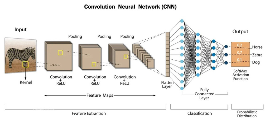
Convolutional Neural Networks (CNN) in Pytorch
A convolutional neural network (CNN) is a type of feedforward neural network that learns features via filter (or kernel) optimization.
When working with images, text, audio etc. data can be loaded into numpy arrays and the can be converted to torch.*Tensor. CIFAR-10 dataset: It has 10 classes, all images are 3-channel of size 32x32 pixels. torchvision datasets are PILImage images of range [0,1]. They are normalized to tensors of normalized range [-1,1].
import torch
import torchvision
import torchviz
import matplotlib.pyplot as plt
import numpy as np
Load and Normalize Data
# Compose - to chain multiple transformations together
# ToTensor - converts a PILImage or a numpy array to tensor
# Normalize - normalizes a tensor image with mean and standard deviation,
# here the mean (0.5, 0.5, 0.5) and standard deviation (0.5, 0.5, 0.5) means,
# subtract 0.5 from each channel and divide each channel with 0.5 to normalize the range in [-1, 1].
transform = torchvision.transforms.Compose(
                [torchvision.transforms.ToTensor(),
                 torchvision.transforms.Normalize((0.5, 0.5, 0.5), (0.5, 0.5, 0.5))]
            )

batch_size = 4

trainset = torchvision.datasets.CIFAR10(root='./data', train=True, download=True, transform=transform)
trainloader = torch.utils.data.DataLoader(trainset, batch_size=batch_size, shuffle=True, num_workers=2)
testset = torchvision.datasets.CIFAR10(root='./data', train=False, download=True, transform=transform)
testloader = torch.utils.data.DataLoader(testset, batch_size=batch_size, shuffle=True, num_workers=2)

classes = ('plane', 'car', 'bird', 'cat', 'deer', 'dog', 'frog', 'horse', 'ship', 'truck')
Plot Images
# function to show an image
def imshow(img):
    img = img / 2 + 0.5 # unnormalize
    npimg = img.numpy() # convert tensor to numpy array
    plt.imshow(np.transpose(npimg, (1,2,0)))
    plt.show()

# get some random training images
dataiter = iter(trainloader)
images, labels = next(dataiter)
# show images
imshow(torchvision.utils.make_grid(images))
# print labels
print(''.join(f'{classes[labels[j]]:5s}' for j in range(batch_size)))
bird plane frog dog

The CNN Model
Convolutional layers preserver the spatial structure of the image. The size of the kernel or filter or 2D patch is called the receptive field, meaning how large a portion of the image it can see at a time. Ouputs after applying convolution are called feature maps. The pooling layers downsample the feature maps, even the pooling layers have a receptive field. Incase of avg. pooling they take the avg. or incase of max pooling the maximum over all values in the patch. Fully connected layers are the final layers, they take features from previous layers to produce predictions. Incase of classification the output of last layer is equal to the number of available classes and this last layers produces probabilities for each class through a softmax function. \[ \mathrm{softmax}(\mathbf{z})_i \;=\; \frac{\exp(z_i)}{\sum_{j=1}^{K}\exp(z_j)} \qquad (i = 1,\dots,K) \]
class Net(torch.nn.Module):
    def __init__(self):
        super().__init__()
        self.convolution_layer_1 = torch.nn.Conv2d(3, 6, 5) # torch.nn.Conv2d(in_channels, out_channels, kernel_size)
        self.maxpooling_layer = torch.nn.MaxPool2d(2, 2) # torch.nn.MaxPool2d(kernel_size, stride)
        self.convolution_layer_2 = torch.nn.Conv2d(6, 16, 5)
        self.fully_connected_layer_1 = torch.nn.Linear(16 * 5 * 5, 120)
        self.fully_connected_layer_2 = torch.nn.Linear(120, 84)
        self.fully_connected_layer_3 = torch.nn.Linear(84, 10)

    def forward(self, x):
        x = self.maxpooling_layer(torch.nn.functional.relu(self.convolution_layer_1(x)))
        x = self.maxpooling_layer(torch.nn.functional.relu(self.convolution_layer_2(x)))
        x = torch.flatten(x, 1) # flatten all dimensions except batch
        x = torch.nn.functional.relu(self.fully_connected_layer_1(x))
        x = torch.nn.functional.relu(self.fully_connected_layer_2(x))
        x = self.fully_connected_layer_3(x)
        return x

net = Net()
Loss Function and Optimizer
criterion = torch.nn.CrossEntropyLoss() # Classification Cross-Entropy loss
optimizer = torch.optim.SGD(net.parameters(), lr=0.001, momentum=0.9) # SGD with momentum
Training the Network
device = torch.device('cuda:0' if torch.cuda.is_available() else 'cpu')
print(f'Device: {device}')
net.to(device)
for epoch in range(2): # training for 2 epochs
    running_loss = 0.0
    for i, data in enumerate(trainloader, 0):
        # get the data; list of [inputs, labels]
        inputs, labels = data[0].to(device), data[1].to(device)
        # zero the parameter gradients
        optimizer.zero_grad()
        # forward + backward + optimize
        outputs = net(inputs)
        loss = criterion(outputs, labels)
        loss.backward()
        optimizer.step()
        # print statistics
        running_loss += loss.item()
        if i % 2000 == 1999: # print every 2000 mini-batches
            print(f'[Epoch: {epoch + 1}, Iteration: {i + 1:5d}] loss: {running_loss / 2000:.3f}')
            running_loss = 0.0

print('Finished Training')

PATH='./cifar_net.pth'
torch.save(net.state_dict(), PATH)
Device: cuda:0
[Epoch: 1, Iteration:  2000] loss: 2.169
[Epoch: 1, Iteration:  4000] loss: 1.830
[Epoch: 1, Iteration:  6000] loss: 1.659
[Epoch: 1, Iteration:  8000] loss: 1.570
[Epoch: 1, Iteration: 10000] loss: 1.513
[Epoch: 1, Iteration: 12000] loss: 1.468
[Epoch: 2, Iteration:  2000] loss: 1.407
[Epoch: 2, Iteration:  4000] loss: 1.374
[Epoch: 2, Iteration:  6000] loss: 1.378
[Epoch: 2, Iteration:  8000] loss: 1.336
[Epoch: 2, Iteration: 10000] loss: 1.297
[Epoch: 2, Iteration: 12000] loss: 1.294
Finished Training
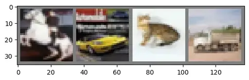
Testing on Unseen Data
dataiter = iter(testloader)
images, labels = next(dataiter)

# print images
imshow(torchvision.utils.make_grid(images))
print('Ground Truth: ', ' '.join(f'{classes[labels[j]]:5s}' for j in range(4)))

# load save model
net = Net()
net.load_state_dict(torch.load(PATH))

outputs = net(images)
_, predicted = torch.max(outputs, 1)
print('Predicted: ', ' '.join(f'{classes[predicted[j]]:5s}' for j in range(4)))

correct = 0
total = 0
# since we're not training, we don't need to calculate the gradients for our outputs
with torch.no_grad():
    for data in testloader:
        images, labels = data
        # calculate outputs by running images through the network
        outputs = net(images)
        # the class with the highest probability is what we choose as prediction
        _, predicted = torch.max(outputs.data, 1)
        total += labels.size(0)
        correct += (predicted == labels).sum().item()
print(f'Accuracy of the network on the 10000 test images: {100 * correct // total} %')

# prepare to count predictions for each class
correct_pred = {classname: 0 for classname in classes}
total_pred = {classname: 0 for classname in classes}

# again no gradients needed
with torch.no_grad():
    for data in testloader:
        images, labels = data
        outputs = net(images)
        _, predictions = torch.max(outputs, 1)
        # collect the correct predictions for each class
        for label, prediction in zip(labels, predictions):
            if label == prediction:
                correct_pred[classes[label]] += 1
            total_pred[classes[label]] += 1

# print accuracy for each class
for classname, correct_count in correct_pred.items():
    accuracy = 100 * float(correct_count) / total_pred[classname]
    print(f'Accuracy for class: {classname:5s} is {accuracy:.1f} %')
Ground Truth: horse car cat truck
Predicted: truck car frog plane

Accuracy of the network on the 10000 test images: 54 %

Accuracy for class: plane is 62.1 %
Accuracy for class: car   is 65.3 %
Accuracy for class: bird  is 40.1 %
Accuracy for class: cat   is 28.6 %
Accuracy for class: deer  is 46.0 %
Accuracy for class: dog   is 53.7 %
Accuracy for class: frog  is 58.8 %
Accuracy for class: horse is 60.4 %
Accuracy for class: ship  is 68.4 %
Accuracy for class: truck is 64.0 %
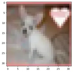
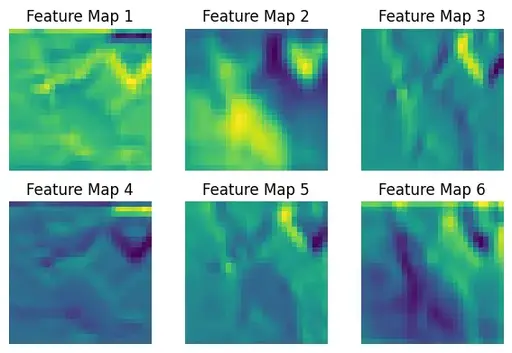
Feature Map Visualization
dataiter = iter(trainloader)
images, _ = next(dataiter)
imshow(torchvision.utils.make_grid(images[0]))
x = images[0]

with torch.no_grad():
    feature_maps = net.convolution_layer_1(x.unsqueeze(0))

#feature_maps = feature_maps.detach().cpu().numpy()
num_feature_maps = feature_maps.shape[1]

fig, ax = plt.subplots(2, 3, figsize=(6, 4), sharex=True, sharey=True)
for i in range(num_feature_maps):
    row, col = i // 3, i % 3
    ax[row, col].imshow(feature_maps[0, i])
    ax[row, col].axis('off')
    ax[row, col].set_title(f'Feature Map {i+1}')

plt.tight_layout()
plt.show()